The intermediate value theorem is of great importance for functions analysis. It notably allows demonstrating that an equation has solutions even if they cannot be expressed. One form of this theorem says: “if a function f is defined and continuous on [a;b] then for every real number c belonging to [f(a);f(b)], the equation f(x) = c admits at least one solution”. The name of the theorem comes from the fact that it shows that all intermediate values c in [f(a);f(b)] are reached when sweeping [a;b].

The Bolzano theorem is proposing a simplified version of the previous theorem. It tells us that “if f(a) and f(b) are of opposite sign, which is equivalent to f(a)f(b) < 0, then the equation f(x) = 0 has at least one solution” (c, which is equal to 0 in this particular case, effectively belongs to [f(a);f(b)]).

The strength of the intermediate and Bolzano theorems is that their assumptions are applicable to all usual functions, which are all continuous at least on a sub-interval of their definition domain.

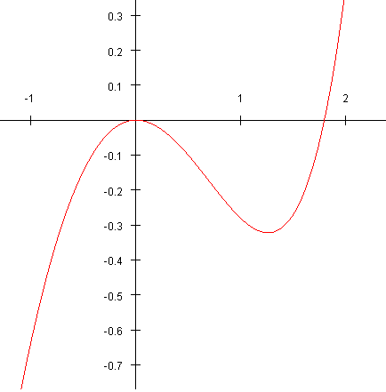
These two theorems can easily be illustrated thanks to graphical representations. For example, let’s consider the function f : x↦e^x-x²-x-1 drawn on the left side. It is easy to show that it is defined and continuous on [-1;2] and that f(-1)f(2) < 0. Consequently, the equation e^x-x²-x-1 = 0 will have at least one solution in [-1;2]. In fact, as highlighted by the curve, there will be two solutions: 0 (evident solution) and a second one which cannot be expressed.

In order to prove the existence of a unique solution in a given interval, it is necessary to add a condition to the intermediate value theorem, known as corollary: “if furthermore the function is strictly monotonic on [a;b] (i.e. strictly increasing or strictly decreasing) then the equation f(x) = c, or f(x) = 0, admits a unique solution. We can for example apply this corollary to our function f: x↦e^x-x²-x-1 on the interval [3/2;2].

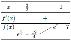The table of variations on the left side effectively shows us that the function f is strictly increasing on [3/2;2] and a calculator gives us easily f(3/2) < 0 and f(2) > 0. Consequently, the equation f(x) = 0 admits a unique solution on [3/2;2].

It is possible to reduce this interval by calculating for example f(7/4),   7/4 being the center of the interval [3/2;2]. The calculator says f(7/4) ≃ -0.058 < 0. Thus, the solution, very often designated as α, is as 7/4 < α < 2. By repeating this method, named  dichotomy, as  many times as needed, it is possible to get as near as wanted from α with the required accuracy. The dichotomy algorithm, which is painful to be run by hand, is usually programmed on a calculator or a computer, allowing getting an approximated value of α with several digits in less than a second. Other more sophisticated methods exist which are converging more quickly (i.e. they require less operations to reach the same accuracy) like Newton’s method of tangents. This method could be detailed in a coming post!